A new adaptive method for both threshold and slope evaluation in the psychophysical experiments is described. This Bayesian method is based on maximizing of the expected information gain (minimizing entropy) on each subsequent trial. The entropy cost function is proven to be insensitive to a particular choice of sampling densities for the threshold and slope parameters, given that they are sufficiently high. The method has been shown experimentally to exhibit the predicted convergence rates and robustness to mistakes at the beginning of the experiment.

 

Introduction

The majority of experimental psychophysical studies involve the measurement of sensitivity for some predefined stimulus or set of stimuli. This requires a technique that specifies the intensity at which each stimulus is just detectable, known as the sensitivity threshold for that stimulus. The threshold is only a part of the story because the transition from non-detectability to detectability is not abrupt; it occurs over some finite intensity range. The stimulus is first detected at some low probability, then with increasing probability until it reaches a high enough level to be seen on 100% of trials. This transition range is captured by the psychometric function relating the probability of correct detection with the stimulus intensity, when represented in log d' versus log contrast coordinates (Fig. 1). The slope of this function reflects the width of the transitional range; the threshold defines its absolute position along the intensity axis. In this example, the slope has a typical value of 3.

Most experimental studies avoid the issue of slope because its measurement is too laborious. They assume a characteristic slope based on past experience. This practice may be hazardous in studies that use common adaptive methods designed for a typical slope value of about 3 (Pelli, 1987a). Often the actual slopes deviate markedly from that assumed value (see, for example, Legge et al., 1987, and Mayer & Tyler, 1986), which make the measurements less precise and subject to systematic errors. In avoiding the slope issue, many studies miss valuable information about the sensory processing such as transducer nonlinearities (Foley & Legge, 1981) and uncertainty effects (Pelli, 1985), which may both strongly affect the slope value. It is important, therefore, to use an experimental method that would efficiently measure the threshold for any slope and measure the slope value, at the same time. Here we describe an adaptive staircase algorithm called the Method that measures both the threshold and the slope in the most efficient manner, given the constraints of randomization of the choice variable.

Any adaptive method for estimating psychophysical parameters needs to address three major issues: estimation of the psychometric parameters (threshold and slope), the termination rule, and placement of the next trial. To do so, it follows the Bayesian principle of taking into account all previous responses to the stimulus in determining the stimulus level for the next trial so as to maximize the information obtained from the response on this trial.

Fig. 5.1. Psychometric function of the probability of a correct response in a two-alternative method, where the mean probability of correct at zero stimulus intensity is 0.5.

 

Estimation

The most efficient way to get the threshold estimate from the results of the completed trials is to keep updating the posterior probability distribution for the sampled thresholds based on Bayes' theorem (Hall, 1968; Watson & Pelli, 1983). The posterior probability distribution is the distribution of probability correct at each stimulus level that has been used so far. The best threshold estimate on any trial is the mean of this distribution (Emerson, 1986) because it minimizes the variance of the threshold estimate (Gelb, 1982, p. 103) and is proven to be more stable than the maximum rule (Emerson, 1986). To keep track of both thresholds and slopes, the posterior probability distribution has to be two-dimensional, where each pair of slope and threshold parameters is associated with some probability (King-Smith et al.,1985). Evaluation of this two-dimensional posterior probability distribution is the core of the Method.

 

Termination Criterion

A purist approach to termination rule would be to evaluate the expected error from the posterior probability distribution and terminate the experiment when the estimated error goes below a certain level. The confidence interval, as suggested by Treutwein (1995), can be obtained by truncation of the left and right tails of the posterior distribution as their areas reach a value of , where is the confidence level. This is a straightforward and computationally inexpensive method.

Watson and Pelli (1983) proposed a different approach for estimation of the confidence interval based on likelihood-ratio test. A further development of this approach was provided by Laming & Marsh (1988), who proposed an approximation formula to compute the variance.

Another possible termination rule is to stop the experiment after a certain number of trials is completed. This rule may be not as efficient as the previous two but it has the advantage of certainty, which is important in the psychophysical milieu (Watson & Pelli, 1983). In our experience observers have difficulty in distributing their effort evenly along an experimental run when the duration of experiment varies. The error of the adaptive method with termination after a fixed number of trials can be obtained by repeating measurements 3-4 times (which is always wise to do) or from the results of computer simulations of the method, such as in Fig. 1 below. For the sake of practicality, therefore, the Method terminates the experiment based on a particular number of trials.

 

Placement

Traditionally, adaptive methods place the next trial at the threshold intensity predicted from the completed trials (Watson and Pelli, 1983; Emerson, 1986; King-Smith et al., 1994). This heuristic rule can be tuned to provide the optimal asymptotic convergence rate by a proper setting of the threshold level (Taylor, 1971). Such tuning makes sense when the number of trials is large and the goal is to get a very precise estimate. For short experiments, as will be shown below, this strategy leaves some room for improvement.

The ideal solution for the placement problem would be to scan all possible scenarios of the sequence of placement choices before all subsequent trials and choose the intensity that provides the minimum expected number of steps before a certain level of accuracy is reached (King-Smith et al., 1994). Unfortunately, this approach is computationally intractable because of its exponential complexity. A surrogate "greedy" algorithm, typically used in such cases, makes the estimation tractable by looking ahead a small number of steps.

This limited approach for adaptive psychophysical methods was introduced by King-Smith (1984), whose Minimum Variance Method minimized the expected variance of the posterior probability distribution after completion of the next trial. Later, King-Smith et al. (1994) compared the one-step and two-step ahead search and found no significant advantage for the latter strategy. This result is a clear indication that, for the particular task of variance minimization, the "greedy" search just one step ahead is about as good as an exhaustive search in full depth. The Method therefore adopts the one-step strategy.

Besides near-optimal performance, another advantage of the Minimum Variance Method is that it has an implicit placement rule defined by the variance-based cost function. This feature makes the method highly flexible. The user does not need to bother with the "ideal sweat factor" (Taylor, 1971) or tabulating the numbers in the procedure for each particular experimental paradigm and parameterization of the psychometric function. For every trial, the method finds the optimal test intensity (within the one-step constraint) driven by its own maximization goal.

However, the variance of the posterior probability distribution, which sets this goal for the Minimum Variance Method, cannot be readily expanded to two dimensions because the threshold and slope dimensions are incommensurate with each other. The properties of two-dimensional version of the Minimum Variance Method would depend on arbitrary weights assigned to these dimensions, which, in turn, depend on the sampling rates of the dimensions.

The approach to overcoming the two-dimensional difficulty is to define the cost function for maximization as the entropy of the posterior probability distribution. This entropy specifies how much information is needed to get complete knowledge of the system under study (in our case, the parameters of the psychometric function that controls the observer's responses). This cost function, first suggested by Pelli (1987b) in his Ideal Psychophysical Procedure, is similar to variance since it measures the spread of the posterior probability distribution. Its defining feature is that linear transforms of the variables do not affect the ranking imposed by entropy among distributions (Cover & Thomas, 1991, p. 234). Consequently, the entropy-based placement rule is insensitive to the sampling rates chosen for the dimensions. The Method therefore employs an entropy-based cost function, which is minimized in deciding where to place each successive trial intensity.

To summarize, the Method is a combination of solutions known from previous literature. The method updates the posterior probability distribution across the sampled space of the psychometric functions based on Bayes' rule (Hall, 1968; Watson & Pelli, 1983). The space of the psychometric functions is two-dimensional (Watson and Pelli, 1983; King-Smith & Rose, 1997). Evaluation of the psychometric function is based on computing the mean of the posterior probability distribution (Emerson, 1986; King-Smith et al., 1994). The termination rule is based on the number of trials, as the most practical option (Watson & Pelli, 1983; King-Smith et al., 1994). The placement of each new trial is based on one-step ahead minimum search (King-Smith, 1984) of the expected entropy cost function (Pelli, 1987b).

The three alternative methods for estimating the threshold and slope of the psychometric function : the method of constant stimuli (Fechner, 1860; McKee et al., 1985), APE (Watt & Andrews, 1981) and the method recently proposed by King-Smith and Rose (1997) all have obvious drawbacks relative to the Method. The method of constant stimuli is non-adaptive and inefficient. APE, although adaptive, uses a non-optimal heuristic placement rule based on a sequence of blocked estimates. The King-Smith and Rose (1995) method places trials based on asymptotically optimal solution for slope estimation. There is no evidence, however, that this method is efficient at the beginning of the experiment, when the threshold is unconstrained.

 

Properties of the Method

To use a psychometric method effectively, one needs to have a clear understanding of its convergence properties. These were determined for the Method in simulations based on 100 trials per condition tested (Kontsevich & Tyler, 1999). The relevant parameters are the rate of convergence of the threshold estimate, the slope estimate, and the bias estimate for each parameter. The main question is, when has the staircase converged to a value of sufficient accuracy and stability that the staircase can be terminated with confidence? Fig. 5.2a shows the standard deviation of the threshold estimate as a function of number of trials. The convergence rate depends on the slope value: for steeper slopes the estimates are more precise. Asymptotically, the error of the threshold estimate is reciprocal to the square root of the number of trials, which corresponds to a slope of -0.5 on the log-log plot (the dB units of the error on the logarithmic scale should not be mistaken for a doubly-logarithmic scale, since the residual near zero is essentially linear). For a large number of trials, the standard deviation is proportional to the slope value. For a typical slope of 2 and a desired accuracy of 2 dB (0.1 log10 units, or about 25%), one needs an average of 30 trials.

 

 

Figs. 5.2c and d show that beyond about 60 trials the bias values for both threshold and slope estimates progressively converge toward zero. This feature indicates that asymptotically the Method produces unbiased estimates in the 2AFC implementation. It is important to run at least 100 trials if the bias is to be stabilized. It should be noted that these properties of the Method were validated in an actual psychophysical observer (Kontsevich & Tyler, 1999), validating that perceptual state changes are sufficiently small that a trained human observer can operate in the manner assumed by the simulation.

 

How the Method Works

?The placement strategy of the Method is to gain maximum information at each trial, which results in different placement rules as the staircase progresses. As depicted in Fig. 1, at the beginning of the experiment the method attempts to localize the threshold; its placement strategy is reminiscent of the bisection method (Press et al., 1992, p. 353). After the psychometric function is positioned accurately on the intensity axis, the slope becomes the object of major concern. At this stage the entropy profile takes on a shape with two local minima and the global minimum alternates between them from trial to trial, as shown in Fig. 2. For a large number of trials, these minima are located at the intensities that correspond to the 0.69 and 0.92 probability levels. Focusing on the slope measurement does not mean that the method abandons the threshold evaluation: it continues to improve the threshold estimate as a by-product of the slope acquisition. Apparently, this is the best strategy when the threshold and the slope are already known with some accuracy.

 

 

Fig. 5.3. Entropy profiles (thin curves) in 6 consecutive trials after the method converged to the threshold. The dots on the curves depict the minimum entropy points where the test intensity will be placed in the next trial. The thick line at the bottom shows the actual psychometric function assumed in this computational experiment. The Method places test points approximately at the ends of the linear region in the transitional part of the psychometric function. This strategy is evidently optimal for slope estimation.

It should be noted that we have no proof that the alternation between the two intensities, to which the method converges while estimating the slope, is random. There is a possibility, therefore, that observers, after seeing the intensity of the stimulus in a current trial, may make a correct guess regarding the intensity in the next trial. Nevertheless, we argue that the knowledge of the particular intensity to be presented at any trial does not affect the outcome of the 2AFC task since it does not help discrimination between the test and blank intervals presented in random order.

Effect of the Miss Rate

In our implementation of the Method, the assumed miss rate is arbitrarily set at a conservative level of 0.04; for trained observers it may be smaller. To evaluate the effect of the assumed miss rate on convergence of the method, we carried out simulations at three different miss rates: 0, 0.04 and 0.08. The slope of the psychometric function of the simulated observer was set at 2, while its miss rate matched that assumed by the method. The results presented in Fig. 5.4 indicate that at the beginning of experiment the convergence of the threshold estimate greatly depends on the assumed miss rate; at larger numbers of trials this dependence gradually vanishes. The slope estimate does retain a residual dependence on the miss rate for the number of trials studied.

This result suggests that a special effort should be made to reduce the occurrence of misses. First, if possible, observers with intractably high miss rates should be avoided. Second, the first few trials may be discarded since they may have higher miss rate while settling into the task.

Fig. 5.4. Performance of the Method with assumed miss rates of 0, 0.04 and 0.08. The miss rate for the simulated observer matched the assumed miss rate of the method. The assumed value of the miss rate greatly affects the method efficiency.

 

Threshold Estimate:Comparison with ZEST

?In many experiments the threshold estimate is the only value needed, and an experimenter may not wish to spend an effort to measure slopes. The common Bayesian adaptive methods (QUEST, ZEST) address this constraint: they estimate threshold based on a realistic assumption about the slope value. This assumption is easy to incorporate in the Method by setting the range of slopes at a single value. We call this version the slope-constrained Method versus the unconstrained version where the method estimates a range of slopes (1 decimal log unit in our simulations). Indeed, the prior information carried by the assumption, given that it is valid, should be beneficial for the method's performance. Moreover, as the computational experiment in Fig. 5.5 shows, neither the ZEST method (a modification of QUEST that is the best among popular adaptive methods) nor the slope-constrained Method have any advantage in practice against the more general unconstrained Method, even when the assumed and actual slopes match.

?The slope of the psychometric function in the simulated observer was set at a value of 2; the assumed slopes in ZEST and the slope-constrained Method were set to this value. The other parameters were the same as in the first simulation (Fig. 5.2). In the implementation of ZEST, the test intensity was placed at the 90% point of the estimated psychometric function, which provided the maximum efficiency to this method. (According to our analysis, this point provides the minimum of the ideal sweat factor, Taylor, 1971.) The slope-constrained Method did not require any preliminary settings since the method itself found the optimal intensity to be tested. The results of the simulations are presented in Fig. 5.5.

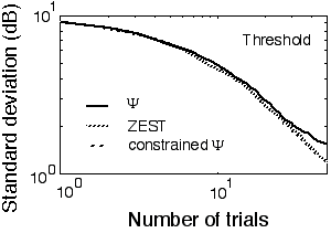
Fig. 5.5. Convergence curves for the slope-unconstrained Method (the slope range is 1 decimal log unit), ZEST, and the slope-constrained Method. The assumed slope in the last two methods matched that in the simulated observer. The placement in ZEST method was at the 90% correct level, the point of maximum efficiency.

The simulated convergence curves for ZEST and slope-constrained Method completely overlapped. This result shows that if the experimenter knows the slope of the psychometric function, the both methods are equally good. The unconstrained Method has practically the same performance with the other two methods up to 30 trials, after which its performance fails to match that of the constrained methods. As already discussed, after 30-40 trials the Method starts measuring slopes and the threshold estimate becomes slope-tolerant. ZEST and the slope-constrained Method continue to take advantage of the prior knowledge of the slope placing optimally at each trial. However, this advantage is based on the shaky ground of the slope assumption. If this assumed slope deviates from the real one, the advantage would disappear since the slope-constraining methods would start making systematic errors and increasing of the trial number would not improve the estimate. There is no such problem with the unconstrained Method.

Each of the methods compared provides the same 2 dB accuracy after 30 trials, which is a typical target level in most psychophysical experiments. The slope-specific adaptive methods have no an advantage over the unconstrained Method within this run length. The mean slope estimate after 250 trials in our empirical evaluation (Kontsevich & Tyler, 1999) was 1.78 + 0.8, which is consistent with other studies (Stromeyer & Klein, 1974; Foley and Legge, 1981). A major complaint of practitioners of Bayesian adaptive methods is that they become unstable if the observer makes a mistake at the beginning of the experiment. To evaluate the robustness of the Method to mistakes at the beginning of the experiment, the observer was instructed to make a mistake on the first trial where the stimulus was clearly visible. The results showed that a mistake at the beginning of the experiment had no significant effect on the convergence of the method. This consistency of the experimental results, together with our experience with the Method applied to other tasks, allows us to conclude that the Method improves the instability problems that haunt earlier adaptive methods.

 

Hardware Requirements

?It would not be an exaggeration to say that modern computer technology has outgrown the extant psychological methods, which use only a small fraction of available computational power and memory. The Method provides a means to harness the enhanced technology to improve the duration and accuracy of psychophysical measurements. At the turn of the millennium, implementing the Method, requires the most powerful personal computers available. The memory requirements of the Method are also quite demanding: for the ranges and the sampling rates used in our simulations the program needs about 1 Mbyte of RAM. Nonetheless, these requirements should rapidly become routine as computing power continues to increase.

 

REFERENCES

Cover, T. M & Thomas, J. A. Elements of Information Theory. New York, Wiley, 1991.

Emerson, P. L. (1986). Observations on maximum likelihood and Bayesian methods of forced choice sequential threshold estimation. Perception & Psychophysics, 39, 151-153.

Fechner, G. T. (1860). Elemente der Psychophysik. English translation: Howes, D. H. & Boring, E. C. (eds.) and Adler, H. E. (transl.), New York: Holt, Rinehart & Winston (1966).

Foley, J. M. and Legge, G. E. (1981). Contrast detection and near-threshold discrimination in human vision. Vision Research, 21, 1041-1053.

Gelb, A. Applied Optimal Estimation. Cambridge MA, M. I. T. Press, 1982.

Hall, J. L. (1968). Maximum-likelihood sequential procedure for estimation of psychometric functions. Journal of the Acoustical Society of America, 44, 370.

King-Smith, P. E. & Rose, D. (1997). Principles of an adaptive method for measuring the slope of the psychometric function. Vision Research, 37, 1595-1604.

King-Smith, P. E., Grigsby, S. S., Vingrys, A. J., Benes, S. C. and Supowit, A. (1994). Efficient and unbiased modifications of the QUEST threshold method: theory, simulations, experimental evaluation and practical implementation. Vision Research, 34, 885-912.

King-Smith, P. E. (1984). Efficient threshold estimates from yes-no procedures using few (about 10) trials. American Journal of Optometry and Physiological Optics, 61, 119P.

Kontsevich LL, Tyler CW (1999) Bayesian adaptive estimation of psychometric slope and threshold. Vision Res. 39:2729-37.

Laming, D. & Marsh, D. (1988). Some performance tests of QUEST on measurements of vibrotactile thresholds. Perception & Psychophysics, 44, 99-107.

Legge G. E., Kersten D. and Burgess A. E. (1987). Contrast discrimination in noise. Journal of the Optical Society of America A4, 391-404.

Mayer, M. J. and Tyler, C. W. (1986). Invariance of the slope of the psychometric function with spatial summation. Journal of the Optical Society of America A3, 1166-1172.

McKee, S. P., Klein, S. A., and Teller, D. Y. (1985). Statistical properties of forced-choice psychometric functions: implications of probit analysis. Perception & Psychophysics, 37, 286-298.

Nachmias, J. & Sansbury, R. V. (1974). Grating contrast discrimination may be better than detection. Vision Research, 14, 1039-1042.

Pelli, D. G. (1985). Uncertainty explains many aspects of visual contrast detection and discrimination. Journal of the Optical Society of America A2, 1508-1532.

Pelli, D. G. (1987a). On the relation between summation and facilitation. Vision Research, 27, 119-123.

Pelli, D. G. (1987b). The ideal psychometric procedure. Investigative Ophthalmology and Visual Science (Suppl.), 28, 366.

Pelli, D. G. and Zhang, L. (1991). Accurate control of contrast on microcomputer displays. Vision Research, 31, 1337-1350.

Press, W. H., Teukolsky, S. A., Vetterling, W. T. & Flannery, B. P. (1992). Numerical recipes in C: the art of scientific computing (2nd edition). Cambridge: Cambridge University Press.

Stromeyer, C. F. and Klein, S. A. (1974). Spatial frequency channels in human vision as asymmetric (edge) mechanisms. Vision Research, 14, 1409-1420.

Taylor, M. M. (1971). On the efficiency of psychophysical measurement. Journal of the Acoustical Society of America, 49, 505-508.

Treutwein, B. (1995). Adaptive psychophysical procedures. Vision Research, 35, 2503-2522.

Watson, A. B. and Pelli, D. G. (1983). QUEST: A Bayesian adaptive psychophysical method. Perception & Psychophysics, 33, 113-120.

Watt, R. J. and Andrews, D. P. (1981). Ape: Adaptive probit estimation of psychometric functions. Current Psychological Reviews, 1, 205-214.